Question

The data file wages contains monthly values of the average hourly wages (in dollars) for workers in the U.S. apparel and textile products industry for July 1981 through June 1987.
a. Display and interpret the time series plot for these data.

b. Use least squares to fit a linear time trend to this time series. Interpret the regression output. Save the standardized residuals from the fit for further analysis.

c. Construct and interpret the time series plot of the standardized residuals from part (b).

d. Use least squares to fit a quadratic time trend to the wages time series. (i.e y(t)=βo+β1t+β2t^2+et). Interpret the regression output. Save the standardized residuals from the fit for further analysis.

e. Construct and interpret the time series plot of the standardized residuals from part (d).

Answer 1

Answer:

a. data(wages)

plot(wages, type='o', ylab='wages per hour')

Step-by-step explanation:

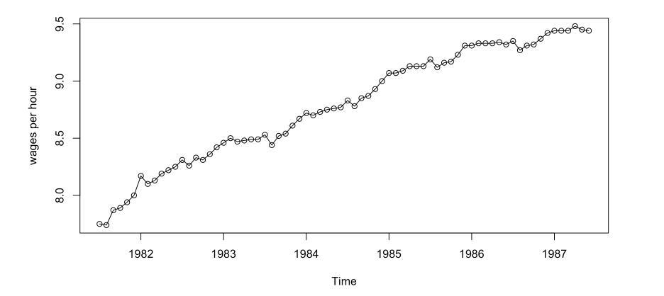
a.  Display and interpret the time series plot for these data.

#take data samples from wages

data(wages)

plot(wages, type='o', ylab='wages per hour')

see others below

b. Use least squares to fit a linear time trend to this time series. Interpret the regression output. Save the standardized residuals from the fit for further analysis.

#linear model

wages.lm = lm(wages~time(wages))

summary(wages.lm) #r square is correct

##  

## Call:

## lm(formula = wages ~ time(wages))

##  

## Residuals:

##      Min       1Q   Median       3Q      Max  

## -0.23828 -0.04981  0.01942  0.05845  0.13136  

##  

## Coefficients:

##               Estimate Std. Error t value Pr(>|t|)    

## (Intercept) -5.490e+02  1.115e+01  -49.24   <2e-16 ***

## time(wages)  2.811e-01  5.618e-03   50.03   <2e-16 ***

## ---

## Signif. codes:  0 '***' 0.001 '**' 0.01 '*' 0.05 '.' 0.1 ' ' 1

##  

## Residual standard error: 0.08257 on 70 degrees of freedom

## Multiple R-squared:  0.9728, Adjusted R-squared:  0.9724  

## F-statistic:  2503 on 1 and 70 DF,  p-value: < 2.2e-16

c. plot(y=rstandard(wages.lm), x=as.vector(time(wages)), type = 'o')

d. #we find Quadratic model trend

wages.qm = lm(wages ~ time(wages) + I(time(wages)^2))

summary(wages.qm)

##  

## Call:

## lm(formula = wages ~ time(wages) + I(time(wages)^2))

##  

## Residuals:

##       Min        1Q    Median        3Q       Max  

## -0.148318 -0.041440  0.001563  0.050089  0.139839  

##  

## Coefficients:

##                    Estimate Std. Error t value Pr(>|t|)    

## (Intercept)      -8.495e+04  1.019e+04  -8.336 4.87e-12 ***

## time(wages)       8.534e+01  1.027e+01   8.309 5.44e-12 ***

## I(time(wages)^2) -2.143e-02  2.588e-03  -8.282 6.10e-12 ***

## ---

## Signif. codes:  0 '***' 0.001 '**' 0.01 '*' 0.05 '.' 0.1 ' ' 1

##  

## Residual standard error: 0.05889 on 69 degrees of freedom

## Multiple R-squared:  0.9864, Adjusted R-squared:  0.986  

## F-statistic:  2494 on 2 and 69 DF,  p-value: < 2.2e-16

#time series plot of the standardized residuals

plot(y=rstandard(wages.qm), x=as.vector(time(wages)), type = 'o')

wages.qm = lm(wages ~ time(wages) + I(time(wages)^2))

summary(wages.qm)

##  

## Call:

## lm(formula = wages ~ time(wages) + I(time(wages)^2))

##  

## Residuals:

##       Min        1Q    Median        3Q       Max  

## -0.148318 -0.041440  0.001563  0.050089  0.139839  

##  

## Coefficients:

##                    Estimate Std. Error t value Pr(>|t|)    

## (Intercept)      -8.495e+04  1.019e+04  -8.336 4.87e-12 ***

## time(wages)       8.534e+01  1.027e+01   8.309 5.44e-12 ***

## I(time(wages)^2) -2.143e-02  2.588e-03  -8.282 6.10e-12 ***

## ---

## Signif. codes:  0 '***' 0.001 '**' 0.01 '*' 0.05 '.' 0.1 ' ' 1

##  

## Residual standard error: 0.05889 on 69 degrees of freedom

## Multiple R-squared:  0.9864, Adjusted R-squared:  0.986  

## F-statistic:  2494 on 2 and 69 DF,  p-value: < 2.2e-16

e. #time series plot of the standardized residuals

plot(y=rstandard(wages.qm), x=as.vector(time(wages)), type = 'o')